Length and dimension   

And nowadays? The problems connected to curves are still numerous, but are mainly too technical to be explained briefly. One, however, deserves to be described, if only in general terms - that of dimension.

An intuitive notion of dimension says that a body has three dimensions, a surface has two, and a curve has one. In general, this is how things stand. If we accept that a line has one dimension, a curve can always be rectified, meaning that it can be reduced to a straight line without changing its length, and so it also has one dimension.

Let's see things from a slightly different point of view. A curve can be made by taking a segment S and bending it like a wire until it reaches the desired shape. Doing so, any point of the curve provenes from one point of the segment. What is obtained is the curve as a parametric representation of S. In this operation, length can remain unaltered, as it happens bending a wire, or it can vary, as occurs when the segment S is drawn on an elastic surface, and then deformed by stretching this surface. There are, it is true, curves of infinite length, that are obtained by deforming not one segment, but a semiline or the whole line. However it is always possible to reduce them again into the shape of a line, in this case infinite. All these curves are called rectifiables.

But is it really true that any curve can be rectified? The answer depends on what we mean by the term curve. If we abandon familiar curves and take the term in its widest meaning, we may be surprised, as in the case of the curve of Peano, which was discovered by the mathematician from Torino, G. Peano (1858-1932).

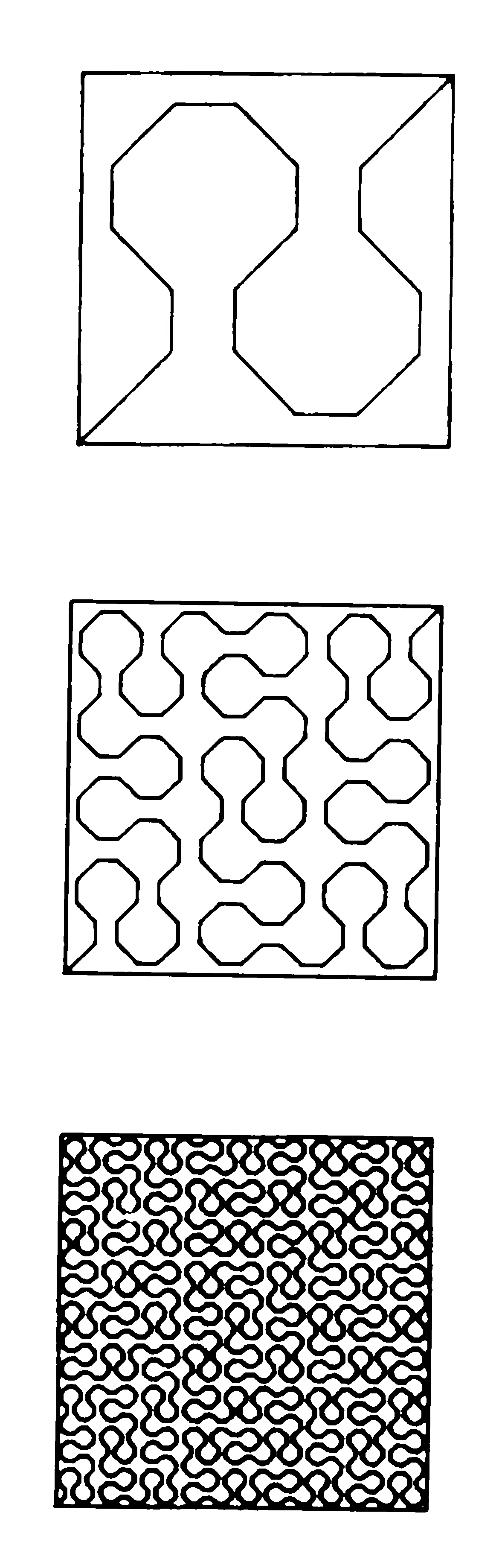
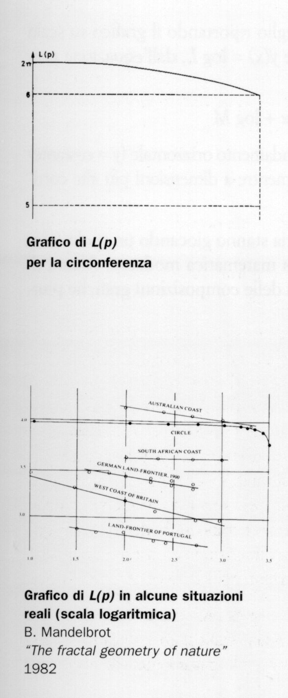
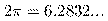
Divide a square into four equal parts, and trace a broken line as in the diagram. This will be the first approximation of the curve. The second approximation is obtained by dividing each square into four squares and replacing the relative parts with more elaborate broken lines. From here onwards the operation is repeated, dividing each square into four each time, and in each of them repeating the substitution.

All these are broken lines, the length of which increases as one proceeds with the subdivision. When the number of the passages tends towards the infinite, the succession of the broken lines "tends" to the curve of Peano. The latter doesn't only have infinite length, as one might imagine, since the length of the approaching liness is always increasing, but it fills all the initial square. The curve of Peano has two dimensions.

The curve of Peano might seem to be one of those obscure concepts often attributed to mathematicians, and in some ways it is, even if helps in clarifying the concept of dimension. In fact, it offers an example of a continuous application between a segment and a square. We owe to G. Cantor (1845-1921), an example of bijective non-continuous application between a segment and a square. He gives two symmetrical examples, that demonstrate that to preserve dimension it is not sufficient just to have either bijective or continuous transformations, nor continuous ones, but that both of these factors are required. In fact, it was demonstrated that dimension is a topological invariant and therefore it preserves itself with bijective and bi-continuous transformations .

These could appear as purely theoretical matters, while the curves encountered in reality behave reasonably "politely"! But nature is not as one might wish. We would like it to be tamed, but the problem of dimension also emerge in situations that appear totally docile at first sight.

Suppose we want to measure the length of a stretch of coast. Because we cannot stretch it until it becomes rectilinear, we will be forced to use some stratagem, which will give us - we hope - at least an approximate measure. Let's take, then, a metre long stick, with an extremity A at the beginning of the piece of coast we want to measure. Then we rotate the stick until the second extremity B touches the coast. This is the first step. From here, we start again by keeping B fixed and rotating the stick until A again follows the line of the coast. This is the second step. With a bit of patience, sooner or later we'll get to the end. Naturally, in order to have an idea of the length we could have used a topographic map and taken steps of - for example - a kilometre. We would have obtained a less precise, but less exhausting, result!

The values that we found are all approximate, having replaced all curves with portions of straight lines. Naturally, the value obtained depends on the length p of the step we take. In other words, we don't have the measure of the coast yet, but a number L(p) varying as the value of P varies. What is expected is that as we use a shorter step, we'll obtain always bigger values of L(p), gradually approaching the "real" value of the length of the coast.

In actual fact this is what happens in some artificial cases, even if the trend of the length L(p) is not as regular as one could imagine. For example, if we imagine a circular island, with a radius of 1km, and report on a graphic the value of L(p) as p varys from 1 km to 1 cm, we have the graphic figure. When p becomes very small, the value of L(p) is close to the length of the circumference km. Not only that, but it is enough to have quite big values of p to get good approximations. With p=1km we already have L=6km. (the inscribed hexagon), with p=100m we have L=6.2806. If then, we assume that p=1m we find L=6.2832.

The same occurs with other regular figures, but when we have to measure real objects, we may be surprised. As p becomes smaller, the number L(p) keeps increasing and does not seem to converge towards a finite value. However, from empirical diagrams L(p) seens to behave as a negative power of p:

The number D, which appears in the previous formula, and obviously depends on the figure in question, is called the dimension of Hausdorff in honour of the German mathematician F. Hausdorff (1868-1942). For rectifiable curves, such as the circumference or conic sections, the result is D=1 and L(p) approaches the length of the curve. In other cases, D is a number higher than 1, even fractionary or irrational.

Naturally it is not possible to demonstrate that a given object in the real world (our coast for instance) has a dimension other than 1. In fact, the definition of dimension depends solely on what happens for "small" values of p, and in practice we cannot push the measures beyond a kind of limit, because at a certain point there is interference of the atomic structure of the matter that eludes any attempt to measure distances that are too small. But we can state that - at least at possible distances - certain coasts (and even some borders between countries) behave as objects with more than one dimension.

the constant D can be seen better if we report the graphic to a logarithmic scale, if we write x=log p and y(x)=log L(p),

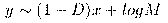
which is the equation of a circle, A horizontal trend (y=constant) characterises the dimension D=1, while more inclined lines correspond to higher dimensions.

Objects with fractional dimensions playing an increasing role in many fields of modern mathematics. Some of them, the fractals, can cause charming graphic compositions to appear.